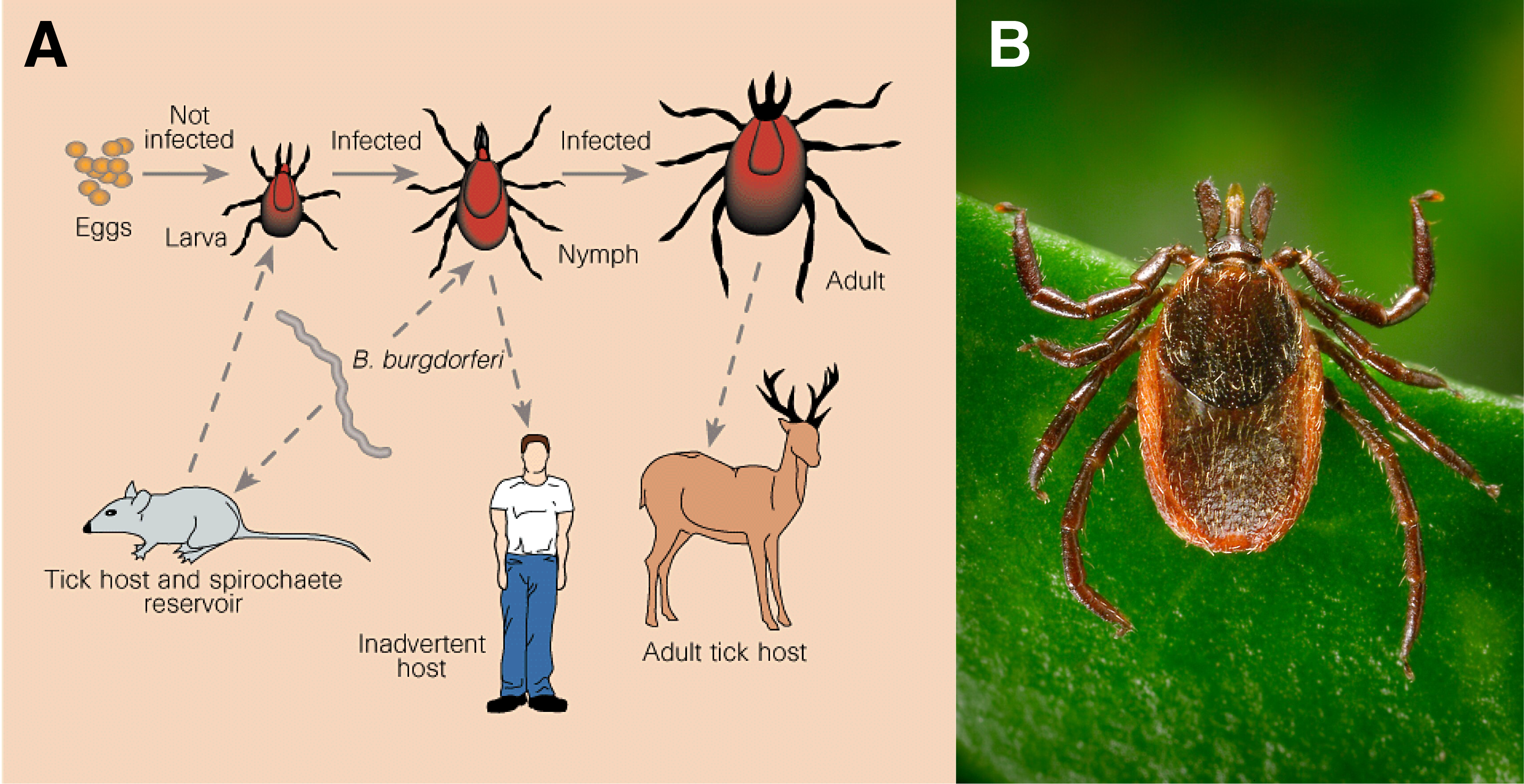
Figure 1. (A) Tick transmission cycle. Barbour & Zückert, Nature 390:553–554 (1997). (B) Adult female western blacklegged tick, Ixodes pacificus. CDC/Loftis et al.
Today’s investigation. Small mammals like mice and squirrels play a central role in the ecology of many forests. As prey, seed dispersers, and disease hosts, they influence both ecosystem structure and public health. In particular, some rodents carry pathogens like Borrelia burgdorferi, the bacterium that causes Lyme disease. Infected ticks that bite these hosts can later transmit the disease to humans. Today, we will use a generalized linear model (GLM) to test how rodent diversity and ecological factors influence densities of infected ticks, which are vectors for Lyme disease, using data generated by the SFSU Swei Lab.
Habitat fragmentation alters the movement and composition of wildlife communities, with cascading effects on the distribution of parasites and the pathogens they carry. In the western United States, the black-legged tick Ixodes pacificus transmits several bacteria, including Borrelia burgdorferi, which causes Lyme disease. These ticks feed on a variety of hosts, including rodents, deer, and predators, and their infection rates are shaped by the diversity and abundance of those host species.
Some pathogens, like B. burgdorferi, rely entirely on horizontal transmission-ticks must feed on an infected host to acquire and later transmit the bacteria. Others, like Borrelia miyamotoi, can be transmitted vertically from tick to offspring. Understanding how these ecological and evolutionary differences interact with landscape features and wildlife communities is key to predicting disease risk.
In this lab, we will test whether the diversity of rodent hosts can help explain the density of B. burgdorferi-infected ticks across forest fragments in Northern California. This is the same question investigated by the Swei Lab at San Francisco State University, which investigates how landscape isolation and wildlife community metrics predict tick-borne pathogen distribution.
Upon completion of this lab, you should be able to:
glmmTMB().References:
Suppose you are studying how the number of bird visits to a feeder changes with outdoor temperature. You observe a series of 10-minute intervals and count how many birds visit a feeder at different temperatures throughout the day. The response variable is a count ; discrete, non-negative, and often right-skewed. Because of this, a linear model (which assumes normally distributed residuals and constant variance) would not be appropriate. Instead, we use a generalized linear model (GLM) with a Poisson distribution, which is designed for modeling count data.
GLMs can be written in the form:
g(μ) = β0 + β1X
where g() is the link function. For Poisson models, this is the log function. This equation says that the log of the expected count (bird visits) is a linear function of the predictor (temperature).
# Fit a Poisson GLM
glm(bird_visits ~ temperature, family = "poisson", data = birds)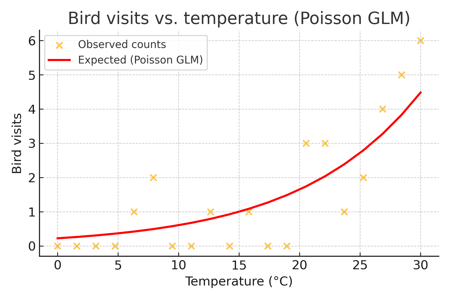
This plot helps illustrate two things. First, count data are right-skewed and discrete. Second, the relationship between temperature and bird visits is curved on the original scale, but linear when viewed on the log scale; exactly what the Poisson GLM models.
To decide which predictors to include, we can compare models using the Akaike Information Criterion (AIC). AIC rewards models that fit the data well but penalizes complexity. The model with the lowest AIC is considered the best among those being compared.
What if the bird visits were measured at multiple times of day in the same location, and we suspected the counts might be correlated by location? In that case, we could use a generalized linear mixed model (GLMM), which allows us to include random effects such as Site or observer. GLMMs are extensions of GLMs that account for grouping or repeated measures in the data.
Stop, Think: Interpret the model output from R (GLM table). Stop and review the Worked example. Think about how you can obtain each value in the model output.
GLMs are most often used when you want to model a response variable that is not continuous and normally distributed. But how do we know if one GLM is better than another? One common method is to use the Akaike Information Criterion (AIC), which balances model fit and complexity. A model with a lower AIC is considered better; it explains more of the variation in the data with fewer or more efficient predictors.
Finally, what if we suspect that observations are grouped, and that there's unmeasured variation across those groups? This is where generalized linear mixed models (GLMMs) come in. GLMMs allow us to include random effects, such as variation by site or subject, which helps us avoid biased estimates. These models are especially useful for repeated measures or nested data; like multiple tick samples taken from the same location.
Now suppose you measured bird visits at multiple feeders, and you think counts might vary by location. You can use a GLMM to include location as a random effect:# Fit a Poisson GLMM
library(glmmTMB)
glmm(bird_visits ~ temperature + (1 | location),
family = poisson, data = birds)ggplot2glmmTMBVariable descriptions: In this lab, we focus on three variables from the dataset. DIN_Bbsl refers to the density of infected nymphs (ticks) carrying Borrelia burgdorferi sensu lato. Rodent_Rich is the number of different rodent species observed at a site. Predator_Shannon_wCat is the Shannon diversity index of predator species (including cats), and Site identifies each sampled location.
Today’s activity on rodent diversity and infected tick density is organized into one main exercise that explores how rodent communities influence tick-borne pathogen dynamics. This exercise will help us apply GLMs to real ecological data, interpret R model outputs, and check model assumptions.
Before we begin fitting models, let’s load the dataset. It contains site-level summaries of tick density, rodent richness, predator diversity, and other ecological variables collected from forest fragments across Northern California. These data were collected repeatedly at each site across multiple years. We'll fit models that account for variation across both sites and years using random effects.
Let’s import the "tick.csv" dataset and explore it.
1a. How many observations and variables?
1b. What type of variable is the response (DIN_Bbsl)?
We are using a Poisson model here because our response variable(tick infection density)is a count. Poisson models are designed for count data that are non-negative integers and often right-skewed. In Poisson GLMs, the variance increases with the mean, which often fits ecological count data better than assuming constant variance and normality.
# Fit GLM with Poisson family
tick_glm <- glm(DIN_Bbsl ~ Rodent_Rich, family = "poisson", data = tick)
summary(tick_glm)Stop and consider: What is the coefficient for rodent richness, and what does it mean? Is it statistically significant?
Let’s interpret R’s glm() summary output.
# GLM output
summary(tick_glm)
Estimate: These are the model coefficients. The intercept gives the expected log count of ticks when rodent richness is zero. The coefficient for rodent_richness tells us how much the log of the expected count changes with each additional rodent species.
Std. Error: This tells us how much uncertainty there is in the coefficient estimate. A large value here suggests the model is less confident in the estimate.
z value: This is the test statistic used to evaluate whether the coefficient is different from zero. It's like a t-value in linear models.
Pr(>|z|): This is the p-value. If it's less than 0.05, we usually consider the effect statistically significant.
Together, these values help us interpret the model and assess which predictors are meaningful.
After fitting a GLM, it’s useful to visualize the model predictions alongside your raw data. To do this, we can use the predict() function, which takes a fitted model and returns predicted values. These predictions can then be added as a new column in our dataset and plotted against the observed data to assess model fit and shape.
# Add model predictions to the dataset
tick$predicted <- predict(tick_glm, type = "response")

# Plot observed and predicted values
ggplot(tick, aes(x = Rodent_Rich, y = DIN_Bbsl)) +
  geom_point(alpha = 0.6) +
  geom_line(aes(y = predicted), color = "red", size = 1) +
  labs(
    x = "Rodent richness",
    y = "Density of infected nymphs (DIN_Bbsl)",
    title = "Predicted vs. Observed: GLM for Infected Tick Density") +
theme_minimal()annotate() or geom_text() to display the model’s AIC or coefficient for rodent richness somewhere on the plot.
After fitting a model, it’s important to assess how well it fits the data. In this step, we’ll visualize the residuals and fitted values to check for overdispersion and other patterns that might indicate poor model fit.
# Diagnostic plots for GLM
plot(tick_glm)2a. What do you see in your plots? Can you spot any trends, outliers, or points that stand out?
The four diagnostic plots from plot() can help you check how well your GLM fits the data. Each one gives you different clues about how your model behaves.
In Chapter 10, we explored how using two explanatory variables together can help reveal interactions or explain more variation in a response. Here, we’ll test whether adding another biologically relevant predictor (predator diversity) improves our model of tick infection density. This step mirrors the idea of exploring multiple factors at once, just as we did with two-way ANOVA.
Stop and consider the original research question and study design. Think about what other biological factors could influence tick infection density, and whether interactions among variables, like those you explored in two-way ANOVA, might reveal new insights.
# Compare two GLMs with AIC
tick_glm2 <- glm(DIN_Bbsl ~ Rodent_Rich + Predator_Shannon_wCat, family = \"poisson\", data = tick)
AIC(tick_glm, tick_glm2)3a. Which model has the lower AIC?
3b. Does predator diversity add meaningful information?
Site as a random effect using glmmTMB() to account for repeated measures and location-specific variation.
Once you've fit the model, compare it to your previous GLM using AIC(). Does accounting for site improve model fit? Interpret your results.
What does your GLMM tell you?
Site or Year. You can think of these as allowing each group to have its own baseline level of tick density.summary() to interpret your fixed effects, and VarCorr() to see how much variation is explained by each random effect.Random effects are especially important when observations are not independent. Ignoring them can lead to overly confident p-values and biased estimates.
Site and Year as random effects. Then use AIC() to compare it with your previous model. Does including both grouping variables improve model fit? Hint: Use summary() and VarCorr() to help interpret your results.
Great Work!
This activity was adapted from the Biostatistics using R: A Laboratory Manual by Raisa Hernández-Pacheco and Alexis A Diaz of California State University, Long Beach by Jenna T. B. Ekwealor for San Francisco State University.

This
work is licensed under a
Creative
Commons Attribution-ShareAlike 4.0 International License.