Phylogenetics

Chapter 14

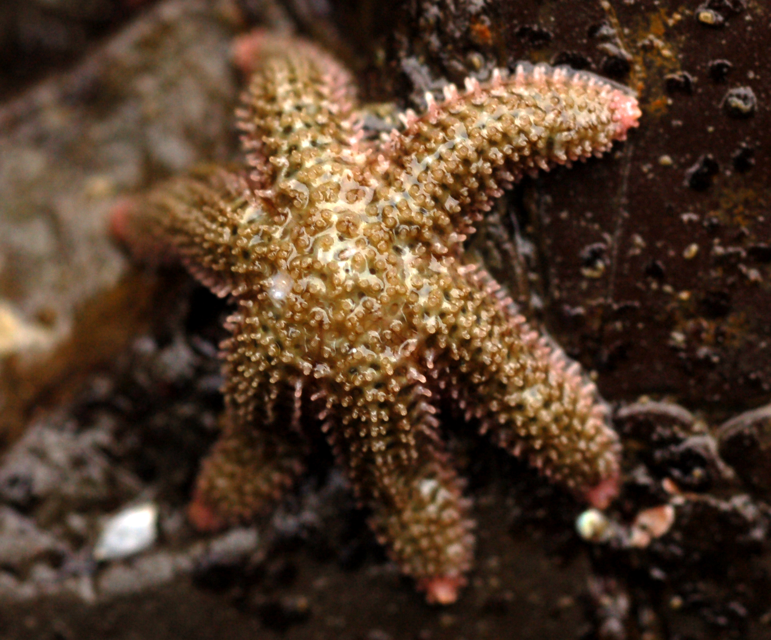
Figure 1. Leptasterias hexactis, a six-rayed sea star. Evolutionary differences may not always be reflected in the morphology, leading to cryptic species. Photo: Matt Knoth via Flickr.

Introduction

Along the Pacific coast of North America, tidepools are home to a group of small sea stars in the genus Leptasterias. These brooding species have limited dispersal and highly structured populations, making them ideal for studying gene flow and isolation. Previous research has found strong population structure across short geographic distances, consistent with limited larval movement. But just how deep is this divergence? Do these patterns reflect population-level structure, or something more?

When organisms show deep genetic differences despite morphological similarity, biologists refer to them as cryptic species. These hidden patterns of diversity are especially common in marine invertebrates, where reproductive isolation and limited dispersal can lead to divergence over relatively small spatial scales. Detecting cryptic species requires molecular tools that can quantify genetic differences and reconstruct evolutionary relationships.

In this lab, we’ll use sequences from the mitochondrial cytochrome c oxidase subunit I (COI) gene, a widely used marker in DNA barcoding and species delimitation. We’ll build and compare phylogenetic trees based on both nucleotide and amino acid alignments. These trees allow us to visualize patterns of divergence and assess whether some lineages may represent reproductively isolated species. Along the way, we’ll learn how to align sequences, build trees in R, and interpret phylogenetic results using maximum likelihood methods.

Upon completion of this lab, you should be able to:

• Construct and assess support for phylogenetic trees using maximum likelihood methods;
• Modify and annotate your phylogenetic tree to produce a useful tree figure;
• Interpret tree topology and bootstrap support in the context of geography and cryptic speciation.

References:

• Melroy and Cohen (2021)

Worked example

Suppose you are studying whether five individuals belong to a single evolutionary group (i.e. a species) or whether they show evidence of divergence. You have DNA sequences from each individual, and you want to use those sequences to explore how closely related they are. We will explore how phylogenetic trees summarize genetic similarity and how maximum likelihood can be used to infer evolutionary relationships.

1. Organize your data

Here are the five sequences from the individuals in your study:

# DNA sequences from five individuals
sequences <- c(
  ind1 = "ATGCCG",
  ind2 = "ATGTCG",
  ind3 = "ATGCCG",
  ind4 = "ATGTCA",
  ind5 = "TTGTCG")

2. Align the sequences

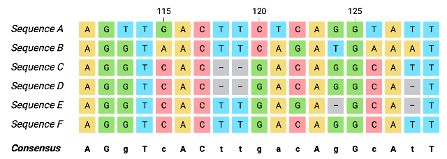
The first step in phylogenetic analysis is to create a multiple sequence alignment. An alignment arranges the sequences so that homologous positions, or sites that share a common evolutionary origin, line up in columns. This allows us to compare characters (like bases or amino acids) across individuals. Sequence alignment algorithms like Needleman-Wunsch or ClustalW score matches, mismatches, and gaps to find an optimal alignment.

Figure 2. A multiple sequence alignment. Gaps are introduced to line up homologous positions across individuals, allowing comparisons across sites.

3. Choose the alignment type

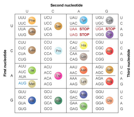
Alignments can be performed using either DNA or amino acid sequences. A nucleotide alignment compares the raw DNA bases directly, preserving all substitutions. A protein alignment translates the sequences and compares the resulting amino acids. This can reduce noise from silent mutations and may better reflect functional similarity when sequences are more divergent.

Figure 3. The amino acids specified by each mRNA codon. Multiple codons can code for the same amino acid, and the third codon position is especially variable. From Smith (2008).

4. Infer a tree using maximum likelihood

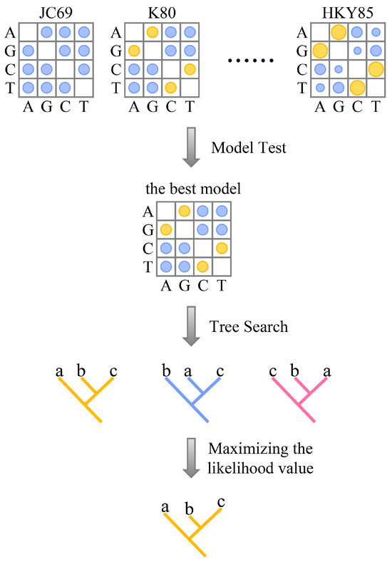
Once the sequences are aligned, we estimate a tree using maximum likelihood. This is a statistical framework that evaluates many possible trees and asks which tree makes our observed alignment most likely, given a model of sequence evolution. A substitution model defines the probabilities of one base changing into another over time. Some models treat all changes as equally likely, while others assign different probabilities to different types of substitutions.

To evaluate each tree, the algorithm calculates the probability of the observed alignment by summing over all possible ancestral states and combining the transition probabilities along each branch. This produces a likelihood score for each candidate tree.

L = P(Data | Tree, Model)

The tree with the highest likelihood is selected as the best estimate of the evolutionary relationships among the sequences. This method considers all sites in the alignment and accounts for both the branching pattern and the amount of change along each branch.

Figure 4. Fundamentals of maximum likelihood method for constructing phylogenetic trees. The abbreviations in the figure are as follows: JC69, the Jukes and Cantor 1969 model; K80, the Kimura 1980 model; HKY85, the Hasegawa, Kishino, and Yano 1985 model; a, b, and c represent different species. Maximum likelihood selects the tree that makes the observed alignment most probable under a given model of sequence evolution. From Zou et al. (2024).

Materials and Methods

• R and RStudio
• Packages: tidyverse, Biostrings, msa, phangorn, ggtree, ape, maps,ggspatial
• Files: coi_nucleotide.fasta, coi_protein.fasta, coi_metadata.csv

File descriptions: This lab uses mitochondrial sequence data from Leptasterias sea stars. The dataset includes:

• coi_nucleotide.fasta: DNA sequences from multiple individuals
• coi_protein.fasta: Translated amino acid sequences from the same gene
• coi_metadata.csv: Specimen information, including locality.

Research question: Does sequence data show evidence of divergence within Leptasterias, and are divergence patterns consistent with geographic structure?

1. Load and align sequences

Start by loading the DNA and protein sequences from the COI gene. These files contain sequence data from Leptasterias individuals collected along the California coast. We'll use R to align the sequences so that homologous sites line up in the same column. This is essential for any phylogenetic analysis: we can only compare changes if we're sure we're comparing the same positions.

# Load sequences
dna <- readDNAStringSet("coi_nucleotide.fasta")

# Align sequences
dna_aln <- msa(dna, method = "ClustalW")

2. Build and compare trees

Now that we’ve aligned the sequences, we can infer a phylogenetic tree. There are many methods, but here we'll be using maximum likelihood. First, we convert each alignment to a format that our downstream phylogenetic software can use. Our output here is a list of aligned sequences, which you can explore to confirm structure.

# Convert aligned sequences to phyDat format
dna_phy <- as.phyDat(msaConvert(dna_aln, type = "seqinr"), type = "DNA")

# View structure in the console
dna_phy

Next, estimate pairwise distances and construct a starting tree using neighbor joining. This gives a rough estimate of relationships based on overall similarity and serves as a starting point for maximum likelihood inference. You encountered distance matrices last week in Chapter 13, where you compared genetic and geographic distances among populations using a Mantel test. Here, we use genetic distances again, this time to construct a tree that summarizes overall sequence similarity among individuals.

# Create initial tree
tree_dna <- NJ(dist.ml(dna_phy))

We then apply a model of sequence evolution to calculate the maximum likelihood tree. This model accounts for how different types of nucleotide substitutions occur over time. For DNA data, we use the GTR model (General Time Reversible), a widely used and flexible model that allows different substitution rates for each pair of nucleotides. This helps improve the accuracy of tree estimation, especially when sequences have evolved under complex patterns of change.

# Maximum likelihood optimization
fit_dna <- optim.pml(pml(tree_dna, data = dna_phy), model = "GTR")

Use ggtree() to visualize and explore the tree. This step is important for identifying patterns or clusters.

# Visualize tree
ggtree(fit_dna$tree) + 
geom_tiplab() + 
ggtitle("Maximum likelihood tree (DNA)")

3. Add bootstrap support

We can assess confidence in the nucleotide tree by adding bootstrap support. Each bootstrap replicate samples the alignment with replacement and estimates a tree. High support (typically >70%) suggests the grouping is consistently recovered.

# Add bootstrap values to tree object
bs_dna <- bootstrap.pml(fit_dna, bs = 100, optNni = TRUE)
tree_bs <- plotBS(fit_dna$tree, bs_dna, type = "none")

# Visualize in ggtree
ggtree(tree_bs) +
  geom_tiplab() +
  geom_text2(aes(label = label), hjust = -0.3) +
  ggtitle("ML tree with bootstrap support (DNA)")

4. Root the tree using an outgroup

To interpret evolutionary direction, we need to root the tree. In this case, we’ll use sequences identified as L. hexactis as the outgroup. These tips should form a clade outside the main group of interest (L. aequalis).

To root the tree, extract the tip labels corresponding to L. hexactis, and use the root() function from the ape package to re-root the tree accordingly.

# View tip labels and identify L. hexactis samples
fit_dna$tree$tip.label

# Re-root the tree on the most recent common ancestor of hexactis tips
rooted_dna <- root(fit_dna$tree, outgroup = ?, resolve.root = TRUE)

# Plot the rooted tree
ggtree(rooted_dna) +
  geom_tiplab() +
  ggtitle("Rooted tree using L. hexactis")

5. Label clades and visualize structure

Once your tree is rooted, the next step is to explore its structure and annotate according to your research question. Each internal node in the tree represents a hypothetical common ancestor. To label clades, you must first identify internal nodes of interest and determine which tips descend from them.

Start by displaying node numbers on your tree:

ggtree(rooted_dna) +
  geom_tiplab(size = 2) +
  geom_text2(aes(label = node), size = 2, hjust = -0.3) +
  ggtitle("Rooted tree with node numbers")

Use these node numbers to define clades. For example, to label all tips descending from node 113 as "Clade X":

# Extract tips from node 113
tips_113 <- tree_subset(rooted_dna, node = 113, levels_back = 0)$tip.label

# Create a data frame that assigns clade to each tip
clade_df <- tibble(tip = tips_113, Clade = "Clade X")

# Plot with color
ggtree(rooted_dna) %<+% clade_df +
  geom_tiplab(size = 2) +
  geom_tippoint(aes(color = Clade), size = 2) +
  scale_color_brewer(palette = "Set1", na.translate = FALSE) +
  ggtitle("Tree with Clade X")

Great Work!